 It doesn’t matter how you make predictions. You can use astrology, economics, meteorology, whatever. Some people even use seasonanality to predict things. For example, there is a view that precious metals go down during the summer months – indeed, they call it “the summer doldrums”. So I thought I would put this theory to the test.
I made use of daily data on silver and gold, going back to early 1968, and I divided each year into three: spring, summer and winter. I then compared the trends. As a measure of trend, I used Pearson’s correlation coefficient. The coefficient ranges from 1 to -1, with a correlation of 1 representing a price that goes up in perfect unison with time, and a correlation of -1 being the opposite. When the correlation is 0, there is no relationship between time and price.
I counted the spring months as January through to May, the summer months June through to August, and the winter months from September through to December – though probably I should have described this last period as the autumn rather than the winter. In other words, the summer doldrums are June, July and August. One can argue about the definition of this period, and some might say that the summer starts on July 4. But already, in early June 2020, many pundits are saying that gold is done for the summer.
Starting off the with silver price, we can set up a box plot, which is based around the median:
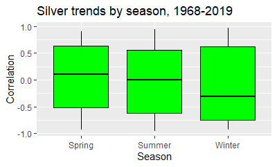
As you can see, the season where silver performs the best is the spring, with a median correlation, between time and price, of +.10. In the three month summer doldrums, the median correlation is -.003, while in the last four months it is -.31. In other words, from a historical perspective the last four months of the year are far and away the the worst.
But are these differences statistically significant? I tested this with a repeated measures test, because I wanted to look at relative performance, by comparing the data within each year. I was not convinced that the data was suitable for a within subjects ANOVA, so I went for its non-parametric equivalent, the Friedman test. By the way, this test was designed by Milton Friedman, which is appropriate, given that the precious metals are supposed to be a hedge against inflation. This test showed that there is no signficant difference between the trends in the three seasons: chi square with two degrees of freedom was 3.23, the p value .20. For completeness I also did three Wilcoxon signed rank tests, comparing the three seasons against each other. None of them were statistically significant.
Then there’s gold. Here’s the box plot:
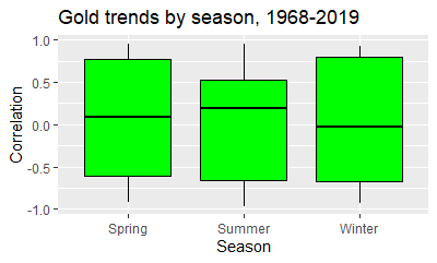
Gold has a median trend of +.08 in spring, +.19 in summer, and -.02 in Winter. In other words, summer is the best performing season, in terms of the median. The mean gives a slightly different picture: +.07 for spring, +.05 for summer and .02 for winter. When we do a Friedman test, we find that there are no signficant differences, with chi square at 2.42, p = .30. Ditto with Wilcoxon signed rank tests.
At this stage, I will concede that there is a problem with the analysis. If you buy gold on June 1, and sell on August 31, and there is a strong upward trend, measured by Pearson’s correlation, this doesn’t mean you have made money. On August 31, just before you sell, the price might crash. We therefore need to consider the absolute movement, across each season.
Here is the box plot of the price changes for silver:
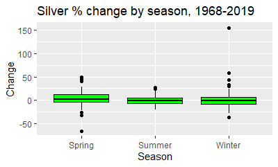
We can see that in the summer there is less excitement, and the winter has some big outliers, with silver going up over 150% one winter. This is reflected in the differences in the means and medians. The seasons have respective medians of 2.56%, -0.54% and -0.89%. Yet the means show a different picture, because of the influence of the outliers: 4.41%, 0.007% and 3.63%. Using the means, we get the first hint that maybe the silver price experience a summer doldrums effect. We can then put the hypothesis to the test, by doing another Friedman’s test. Chi square is 3.5, with two degrees of freedom, and the p value is .174. In other words, it is not statistically significiant. And neither are the Wilcoxon signed rank tests used to contrast the three seasons against each other.
Let’s now move to gold. Here are the box plots:
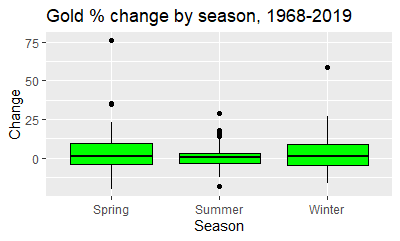
You can see that there is a less volatility in the summer, with the green box, representing the range between the 25th and 75th percentiles, being relatively compressed. The summer months also have the lowest median and mean. The medians are respectively 1.36%, 0.57% and 1.47%, the means 4.02%, 1.25% and 3.31%. Yet the Friedman’s test is not statistically signficant – the chi square is .346, the p value .841. It goes without saying that the Wilcoxon tests were likewise insignificant.
Yes, there is evidence that the price of gold and silver don’t move as much during the summer months. However in terms of directional movement, the theory that the precious metals suffer from a summer doldrums effect is unsupported.